
Instructions
Before commencing, ensure that the monitor and printer are set up as detailed in the Settings page
Overview

Using a densitometer or Stouffer R3705-1 Gray Scale, find the RGB and density values for white and Dmax on the TruNeg gradient.
Then find 10 intermediate densities on the gradient specified by the program, enter the RGB values that produced those densities, and save the preset.
Convert and print the negative, and print the print.
The Details
The TruNeg Gradient

The Gradient is a 128-step logarithmic stepwedge between RGB 8 and 248. It is labelled in “8-bit” notation to three significant figures, and each second step is numbered.
The stepwedge is 14.6 (37.1 cm) inches long to fit the long side of a quarter sheet of watercolour paper. It is 2.14 (5.43 cm) inches wide.
Adjust the size if necessary, but keep it as large as possible. The Gradient can be downloaded from the Downloads page.
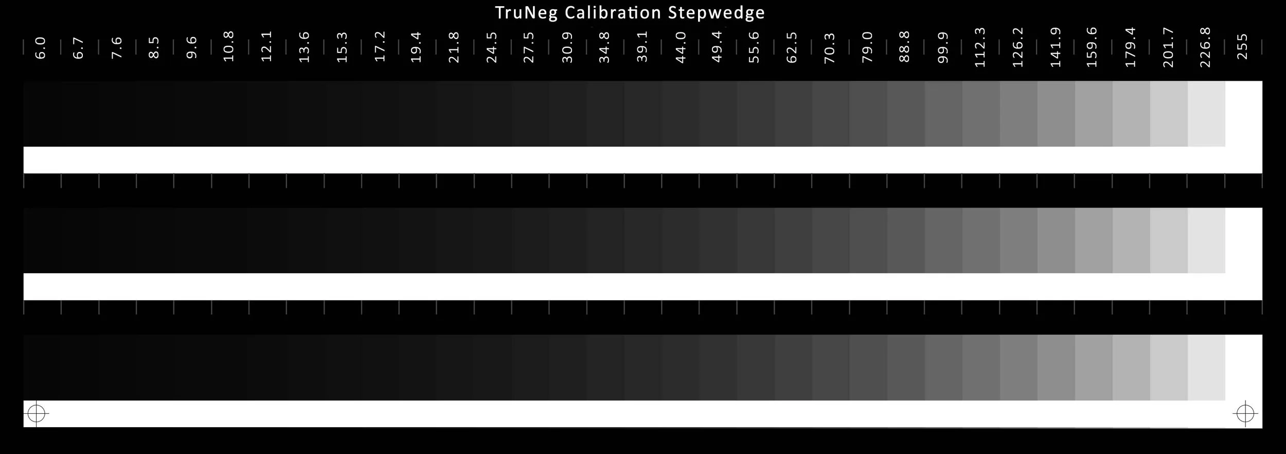
If you do not know the exposure, it is easier to find the RGB “Just White” and “Just Black” points using the 3 ×9 inch Calibration Stepwedge. The stepwedge has three identical stepwedges, making it easy to do, say, a 3-, 6-, or 12-minute test to find a good exposure. If needed, find an intermediate exposure that meets the criteria, noting that there is no perfect exposure, just as long as you have a good Dmax and a clean white.
The Calibration Stepwedge can be downloaded from the Downloads page.
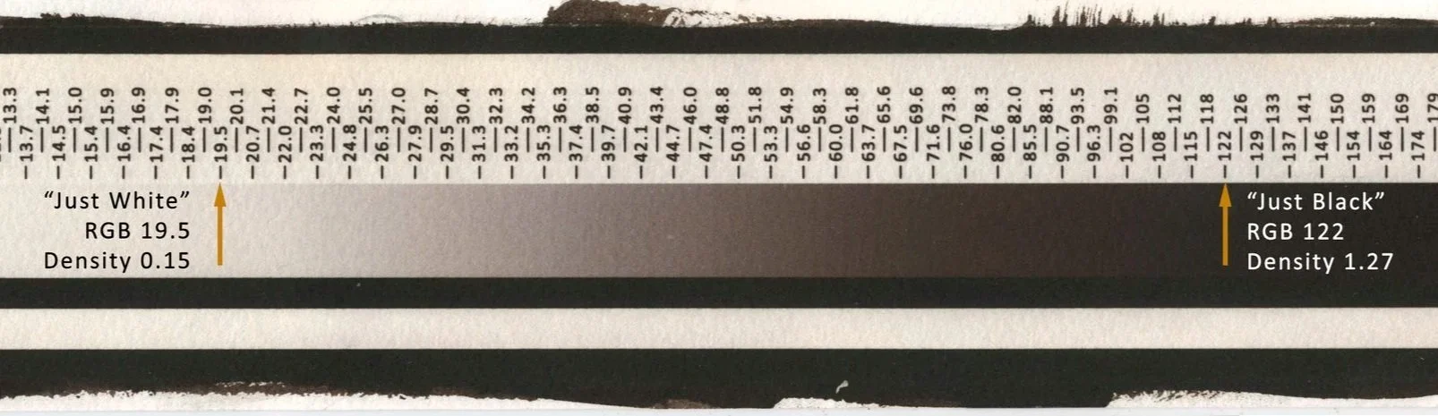
Once the white and Dmax are known, there is no need to print the full gradient.
Keeping the whites of alternative processes stain and fog free can be difficult. The “Just White” point is the last step before the gradient stops getting lighter.
If in doubt, choose the slightly darker step, but be aware that this will be the lightest tone in the print.
The “Just Black” is the last tone that can be separated from the adjacent Dmax strip. Run your finger down the Dmax strip and stop at the first obvious “black” or Dmax point where the gradient merges into the strip. If in doubt, choose the slightly darker step.
This establishes the darkest shadow tone without affecting the maximum density and should be just discernible from Dmax.
Instructions for Densitometer
Instructions for Stouffer Stepwedge
Scan the gradient and Stouffer Stepwedge together at 360 dpi. The scan only needs to look reasonably true, with separation in the gradient shadows and highlights.
In the editing program, convert the scan to B&W, and adjust the Stouffer Stepwedge Dmax to RGB 16 and the white to 250, keeping the gamma at 1.
The gradient’s Dmax will normally appear lighter than the step wedge’s, and the gradient’s white will be darker.
Download and open the 360 dpi Stouffer Density Notation file from the website, copy and paste it beside the stepwedge aligning the numbers with each tone. Note that the first value is the first step wedge tone.
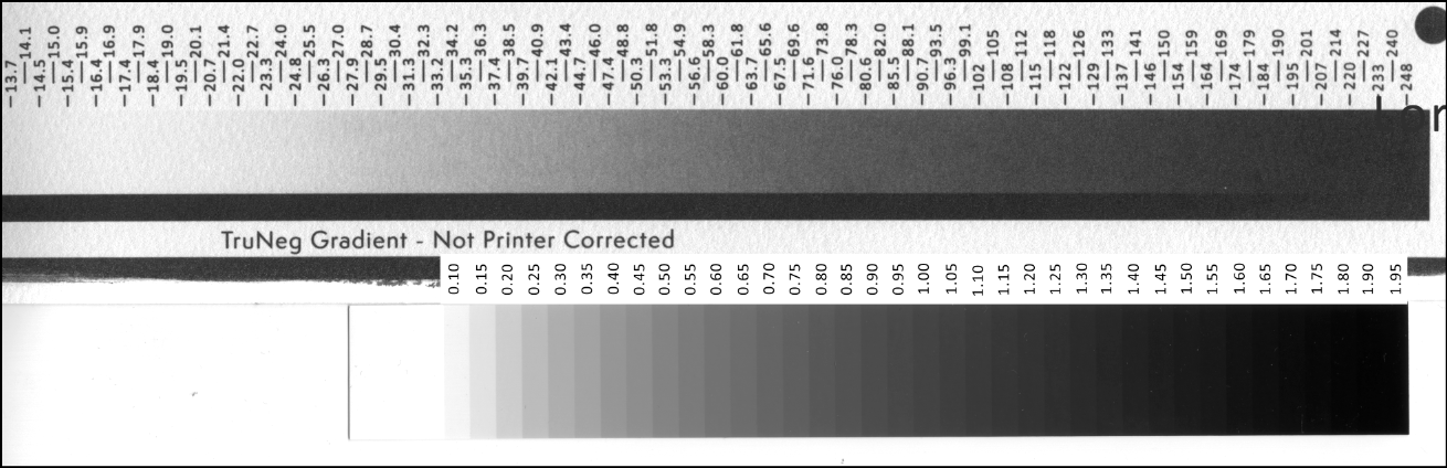
Using the colour picking tool, find the gradient’s RGB value for just white using a sample size large enough to even out the effects of the paper texture, #1 below. Now find the density that best matches that RGB value in the stepwedge, #1A. Enter the RGB and density into the Profiler.
Do the same for the Dmax just black values. #2 and #2A below.
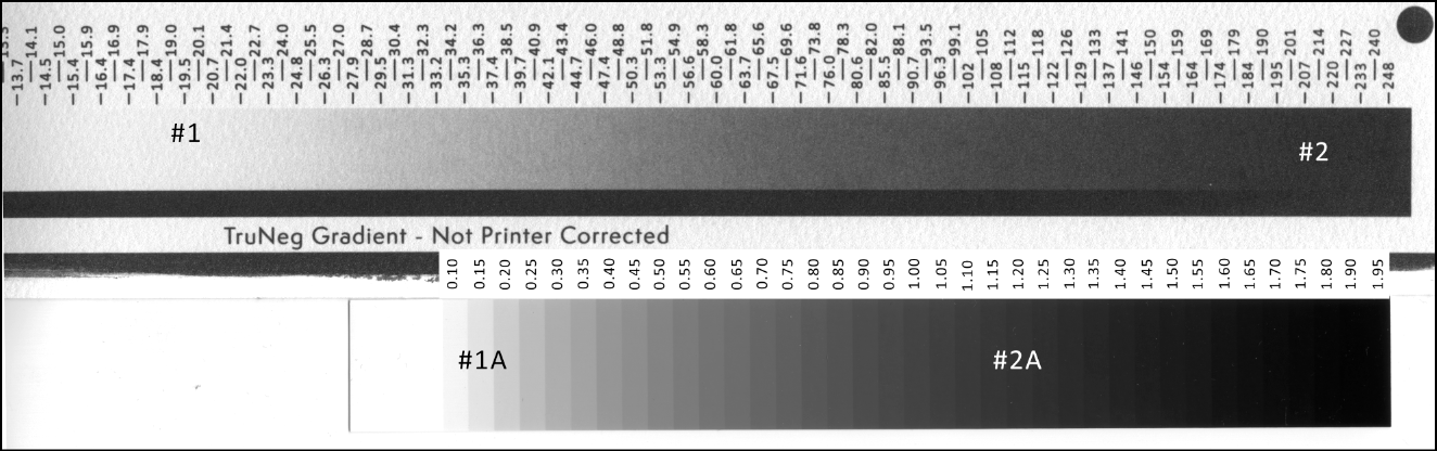
Having decided on the white and Dmax points, measure the densities and enter them with their corresponding RGB values into the Profiler.
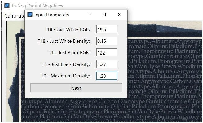
The program calculates ten intermediate target densities and displays them in bold text in the Profiler window. The densitometer is then used to find the densities, and the matching RGB values are entered in the adjacent fields.
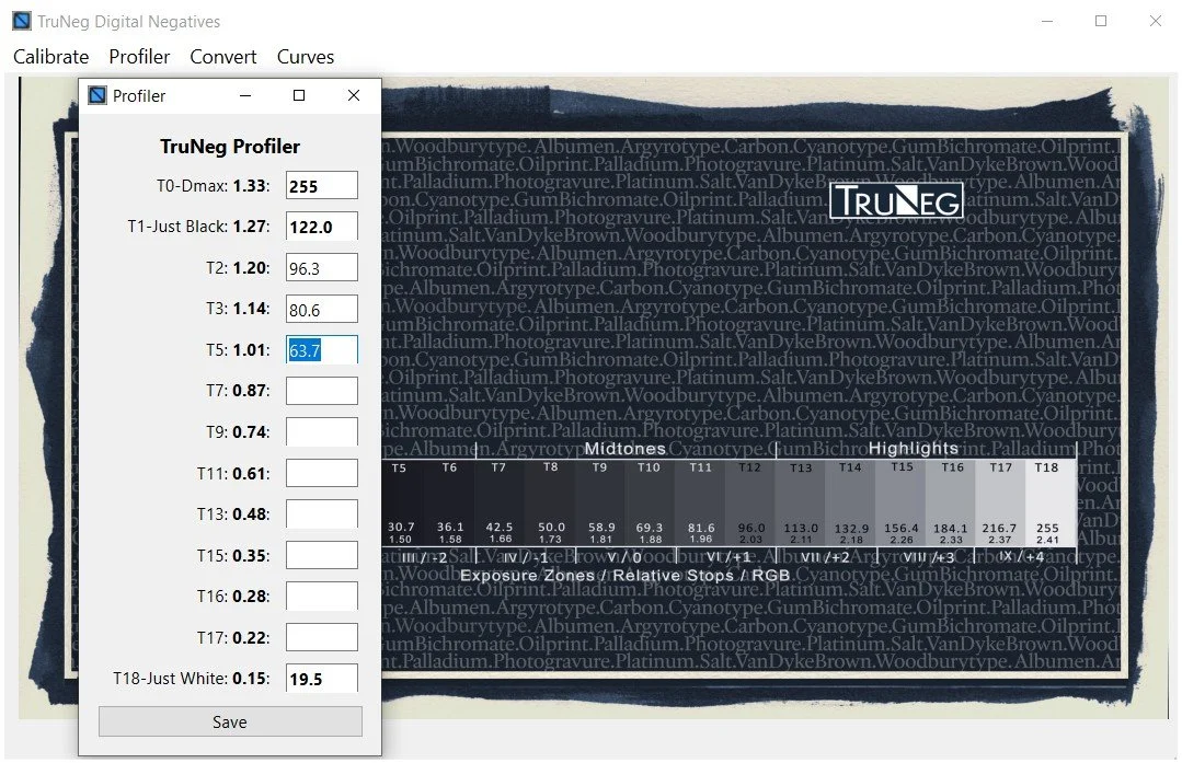
The program calculates ten intermediate target densities and displays them in bold text in the Profiler window shown opposite.
Using the colour picker, find the stepwedge value closest to the densities shown in the Profiler, measure the RGB value and find the same value in the gradient. Enter the gradient RGB value into the Profiler.
For example, if the T2 target density is 1.14, the closest stepwedge density is 1.15, with an RGB value of 58. Locate RGB 58 on the gradient and RGB 159 is the negative value that produced a density of 1.15.
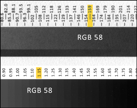
Do the same for each, and when completed, save the file as shown opposite.
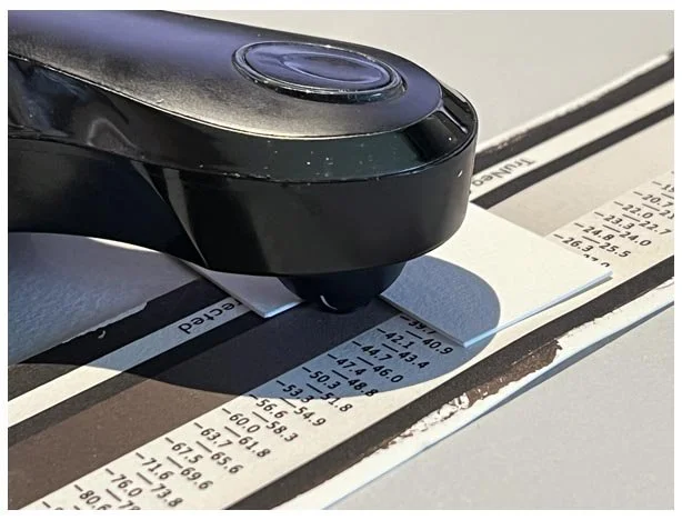
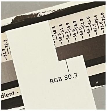
A small piece of card with a notch cut out helps to line up the densitometer.
When completed, save the file identifying the process and exposure time. The program adds the just white and black values, the overall gamma and appends “Profiled” to clearly identify the Preset. The Preset is saved as a Python Pickle file. At the same time, the recorded densities are saved in a separate file.
E.G. Kalli(3).pkl(19,4_121,9_0,665)Profiled
Kall(3)_density.pkl
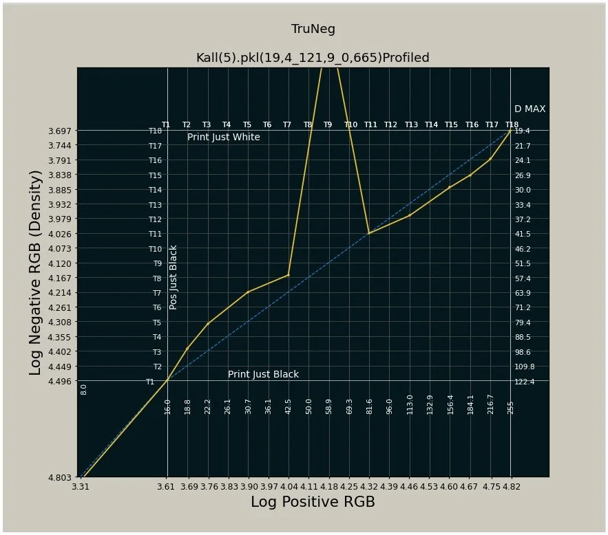
The Preset curve should be viewed before conversion to check for input errors and smooth out any slight wobbles.
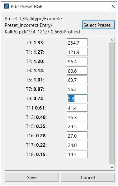
If there is an obvious error, such as a large spike in the curve, open the Edit_RGB menu, select the Preset (not the Density file), find the error and overwrite the entry and save the corrected Preset.
Note that if the curve has been tweaked, the tweak will need to be redone
Convert
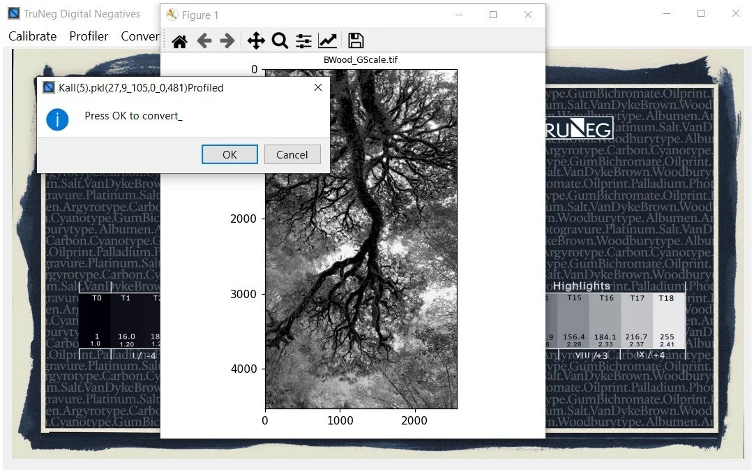
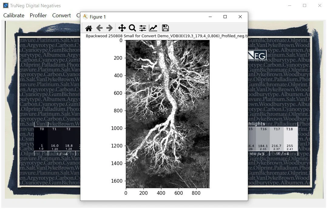
Open the Convert menu, select the image and preset, then press OK.
Once the negative is completed, which can take 30 seconds or more, it is automatically exported to the Preset folder, ready for printing.
Print the Print
If you have confidence in the consistency of your process and the image has been edited on a monitor with a gamma of 1.8, you can go straight to print. Otherwise, make a test strip and, if thought necessary, edit the image with the DLog
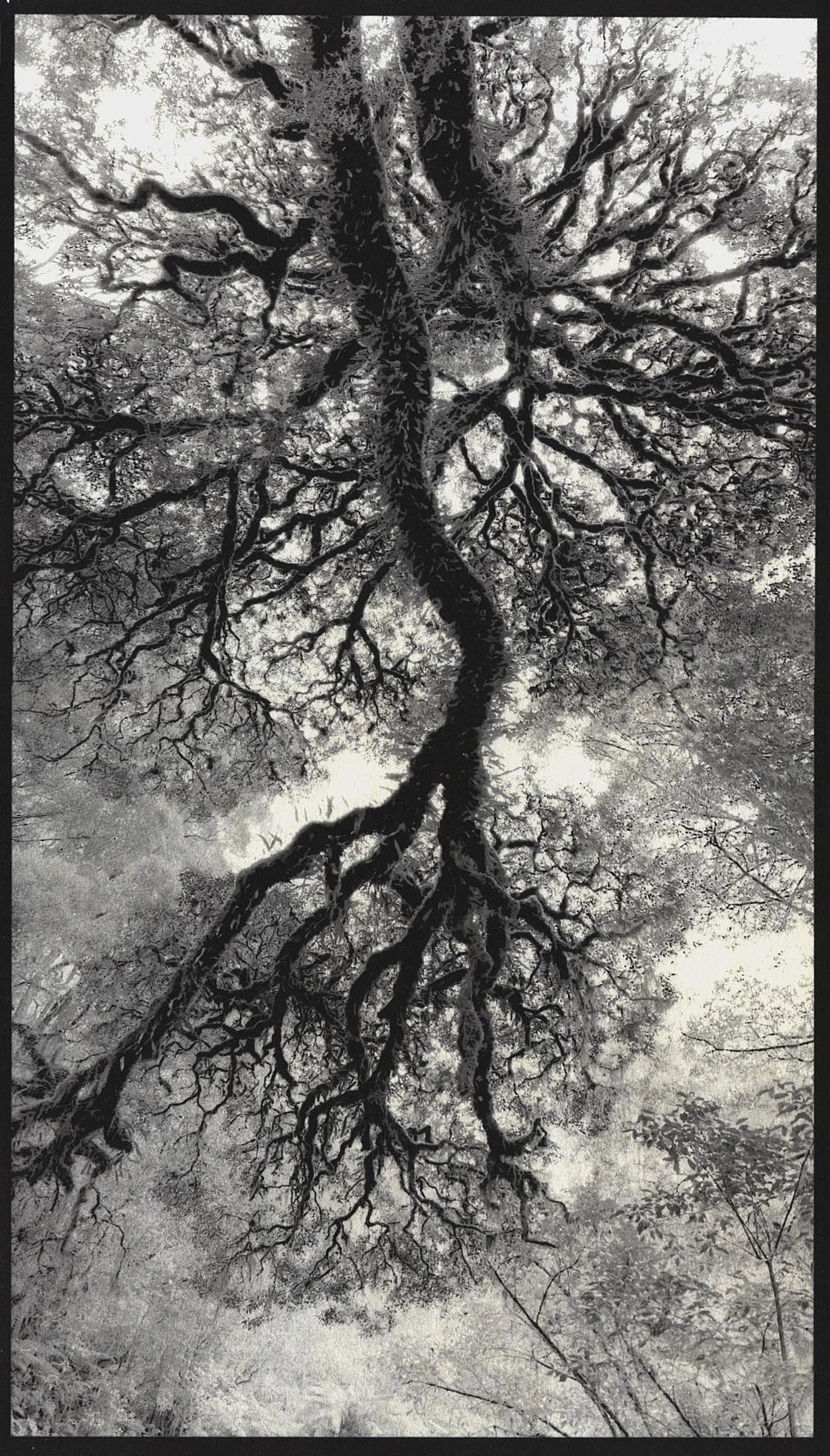
.1×12.5 inch (18×32 cm) Kallitype print made from a profiled negative without further correction. Photograph & print by John Riches